Geiger Counter and Dosimeter

A nice pic from the current state of my Geiger.

Status of Project

Code Repository: https://bitbucket.org/jpcf1/geigerc
Status: Ongoing
Done:

9V-400V Boost DC-DC Converter
Geiger Tube detects background particles, emits current pulses
Pulse-shaping circuit
Microcontroller counts pulses, sends over Serial Port

To-dos:

Add a display, to make it portable
Improve DC-DC efficiency
Refactor code to a micro-kernel architecture, with a task Scheduler
Make a case for it
Order radioactive samples to test it

Overview

As you have probably have guessed from this website, I am really passionate about Physics, and I have a desire to understand how all visible and invisible things work on our Universe. Radioactivity has been a phenomenon that has always stirred my interest. I guess it reminds us of a world that is vaster than the visible and mundane everyday things that bore our everyday life.

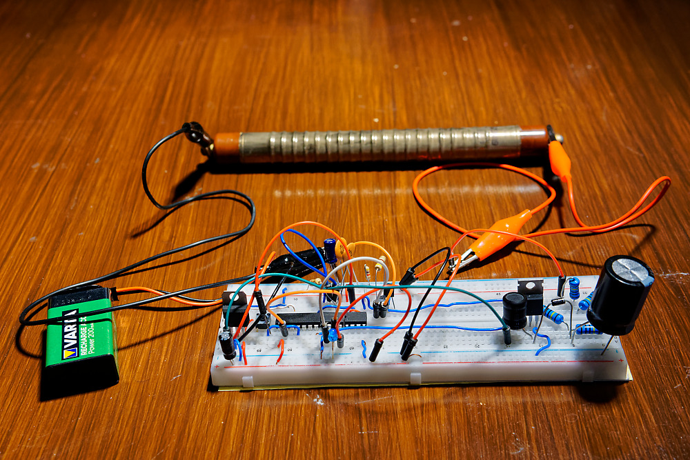
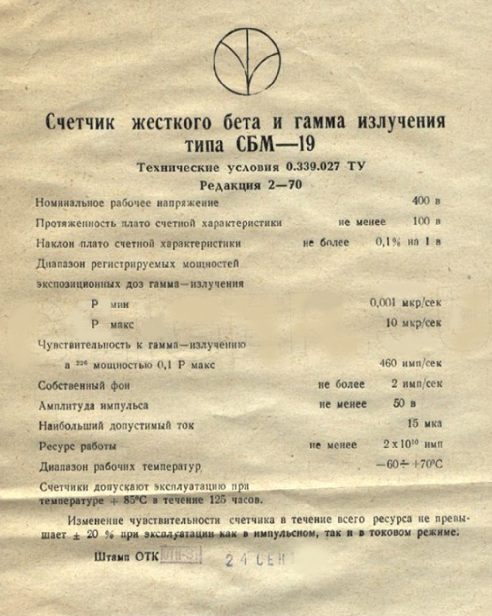
Some time ago I decided to order a Geiger Tube on eBay. It's an SBM-19 tube, which mas made in the former Soviet Union. I went for this one as my first tube, since it is quite sensitive to background radiation, around 80 Counts per Minute (CPM), which means I can already get some "clicks" without the need of radioactive sources.

A Geiger tube is a hollow metallic cylinder, with another metallic rod in the middle, and the interior is filled with a noble gas like Argon or Neon. The metallic rod and the cylindrical shell are kept at very high voltage (around ~400V), just below the electric breakdown voltage of the gas. This way, whenever an ionizing particle/ray enters the tube, it ionizes one of the gas's atoms, causing an avalanche of free electrons which are accelerated by the extremely high electric field established between the cathode and anode. This in turn generates a current pulse, that signals an ionization event.

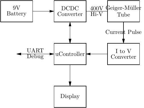
After this brief discussion, we can already have a glimpse of which would be the essential building blocks of a Geiger counter. We need:

A high-voltage generator, to generate 400V from a low voltage source, possibly a 9V battery for portability reasons.
The current pulses need to be converted into a standardized voltage pulse, with consistent properties and shape, so that its edges can consistently toggle a counter.
Some display mechanism, to get readings
A microcontroller, to count the pulses and serve as a flexible platform to implement additional functionalities that might prove useful

The following sections outline how each of these blocks are internally design. In the end, you can see the final result of them operating together in the chapter Operation and Testing, and also the Future Work I have planned.

As previously mentioned, all code can be checked out from the following Git repository: https://bitbucket.org/jpcf1/geigerc

Disclaimer #1: the code is free to use for educational and hobbyist purposes. All commercial exploitation of the code, or parts of it, is strictly forbidden. You can contact me for a license.
Disclaimer #2: this circuit has high voltage nodes, which can be potentially lethal. If you are not skilled enough in electronics, do not attempt to assemble it. If you choose to assemble this circuit, I hereby waive all responsibility on any material or human damage. You do it at your own risk.

The DC-DC Converter

Theoretical Background

So... we need 400V! That's a far away from the 9V battery planned to be used! Well, it may seem like that, but in the end a high voltage simply means that there is a very high electric field between two points, and this is achieved, for instance, by accumulating charge on capacitor plates up to a point where the voltage across them is 100V, or 200V if we charge it a bit more, or 300V if we give it even a bit more.. until we reach our 400V target that sets the Geiger tube in its optimal operation region. Remember that Q=CV, or V=Q/C. And our battery has plenty of charge (Q) accumulated, we just need to find a way to jiggle it from one place to the other!

Okay, just connect the 9V battery to the capacitor, you might say! Well, from elementary circuit theory, the capacitor would asymptotically charge to 9V, so that the potential difference between the battery and the capacitor would match, and therefore no further current would flow into the Capacitor that would charge it to voltages higher than 9V. What we need then is a way to shoot current into the capacitor, regardless of the voltage across its terminals.

One way to achieve this is using a DC-DC Boost converter topology, as can be seen below.

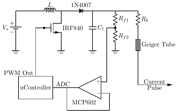
The operation is very simple. As you might know, the voltage across an inductor with inductance L is V = L di/dt, and if we rearrange the equation, we get TODO. In simpler terms, the inductor accumulates current across itself whenever a voltage is applied to it, and the current cannot change instantaneously across its terminals, since the inductor differentiates current, and this would cause a current spike. Therefore, the inductor is the perfect "current pistol" we spoke about before (well, actually more like a current hose!). Consider in the above figure that we apply a Pulse-width Modulation (PWM) signal to the transistor gate.

When turned ON, the transistor connects the inductor to ground. Therefore, ignoring parasitic R, the current rises linearly with V_s to a maximum of I_max = V_s δ T / L, where δ is the duty-cycle and T the period of the PWM signal.

During this period, the Diode is reverse biased, so it will not conduct, behaving as an open circuit. This means that the Capacitor will discharge to the load R_l and, consequently, V_o will decrease a bit. This is the source of voltage ripple.

When turned ON, the transistor is effectively an open circuit, and the inductor will discharge through the diode to the Capacitor (and Load), increasing V_o.

Note that, however, during the first few cycles, V_o is not high enough, so the diode will actually conduct even in the transistor-OFF stage.

LTSpice Simulation

On the folder analog/dcdc, you can find an LTSpice simulation of this circuit, together with a python script that automates the simulation runs. The values used for the components are:

L = 470 μH
C = 47 μH
R_f1 = 1 MΩ
R_f2 = 4.7kΩ
R_b = 4 M Ω

The python script simrun.py launches two LTSpice simulations in parallel threads that simulate two states of the circuit: the startup, and the steady-state phase (when V_o has already reached its target value). Each simulation run has its own .sp file for analysis, where you specify the SPICE analysis commands for each type of run. They are, in turn, configured in a Python dictionary that is parsed by the script. The analysis file in both cases has only one variation, which is the .op operation point setting for a steady-state scenario. In order for the script to run, you simply need to install the ltspice and the matplotlib python packages.

The simulation results are the following:

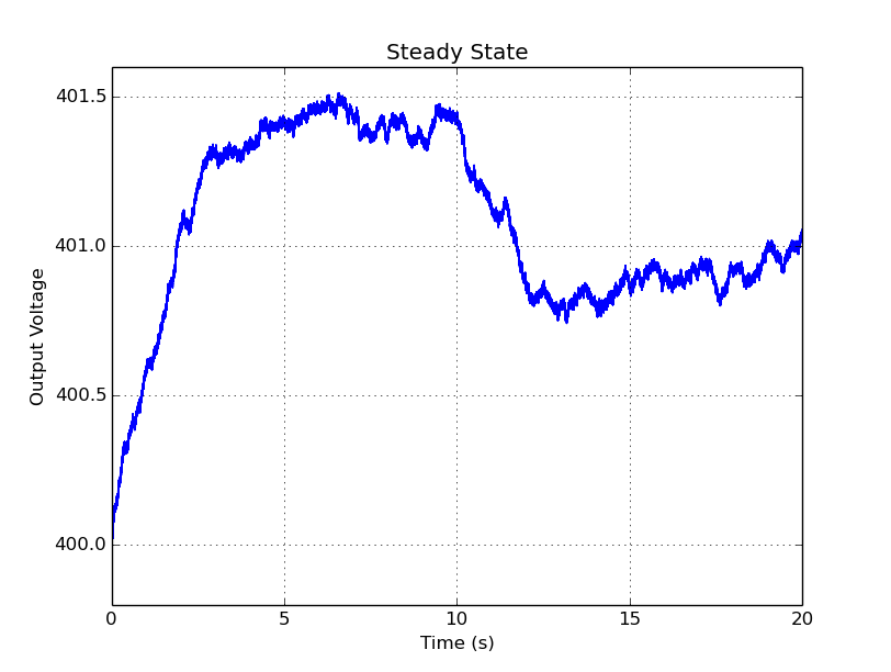
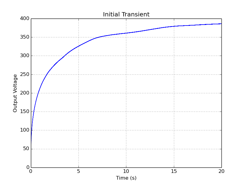
LTSpice simulation - Steady State Operation

Figure 4 - LTSpice simulations of DC-DC Converter, managed and graphed in Python/NumPy.

It takes around 15 seconds for V_o to rise to the operating voltage, but, when in steady-state, the voltage is stable around 401 V, with a ripple voltage of around 700mV. We should note that this simulation is a worst-case scenario, since we have not included the Geiger tube, and the R_b is continuously sinking current to ground. With a Geiger tube however, we would only have 10 μA pulses for each crossing ionizing particle, and otherwise it behaves like an open circuit: this means that the capacitor does not discharge as much (only to the feedback resistors), and therefore the V_o decreases less. This is why we need a feedback control loop, which will be explained further ahead. As can be seen in the analysis_ss.sp and analysis_init.sp files, I have included a few SPICE .meas commands to calculate interesting metrics such as average input and output power, average and peak currents, and so on.

Note #1: since the simulations are lengthy, they can take quite some time, in the order of ~10 minutes. Reduce the simulation time for quicker runs
Note #2: the output .raw files can be quite big (around ~1GB), depending on the length of the simulation.

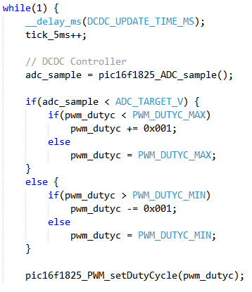
The need for a Feedback Loop

It is important to notice that, when running freely with a given duty-cycle, we can have a potentially instable system, whose output voltage can rise indefinitely until the capacitor explodes! Among other factors, even if we calculate the exact δ and T and leads to a given V_o, the load can vary. If the load increases, the capacitor discharges less during every transistorOFF stage, and therefore the net result can be an increase in V_o, instead of it remaining constant.

There is a very simple remedy for this: negative feedback! For this, we use R_f1 and R_f2 as voltage dividers, that divide V_o suitable to be fed to a microcontroller ADC. The microcontroller can then react on changes in V_o, and lower or increase the δ accordingly, so that less current, or more, is fed to the Capacitor.

The chosen values for R_f1 and R_f2 yield a voltage division factor of 0.004678. This means that for V_o = 400V, V_f ≈ 1.87 V, which is a voltage suitable for a microcontroller ADC, since its reference voltage will be the microcontroller supply voltage of 5V (an LM7805 voltage regulator is used).

Geiger Tube and Pulse Shaping

From the Geiger Tube's Datasheet, and also from circuit measurements using the Soundcard Oscilloscope, I gathered two important facts:

The maximum "dead time" of the tube seems to be somewhere around 200 μs. As the name suggests, it is the period of time, after an ionization event, during which the tube counter becomes unable to respond to another ionizing particle. This effectively limits the maximum counting rate, which should be around 1/(200 μs) = 5000 Counts per Minute (CPM).
The current pulses seem to peak at around 10 μA.

The current pulses can be amplified by a BJT NPN Transistor. We can simply feed the negative end of the tube to the base of the transistor, which then generates a sinking current at the collector of I_c = β I_b, where I_b is in this case the current generated by the tube, and β is a transistor parameter, generally in the order of 100~200. In fact, I ended up using a Darlington Pair composed of two BC547 NPN transistors cascaded. As it is known from theory, this is the equivalent of using a transistor with an equivalent β_eq = β². With this configuration, we are effectively multiplying the current by a factor of around tens of thousands, bringing the current pulse closer to the hundreds of mA range. If we then connect a Resistor to the collector of this transistor pair, with that current, we already get a workable voltage level. Et voilà, we have our current-to-voltage ready!

Okay, now that the pulses coming from the tube are actually noticeable, we need to tackle the final problem of their timing. The "dead time" measurement I presented is actually a maximum value. This means that the pulses can actually be shorter, fainter. This might be okay if you want to see your particles as a blinking led, but timing variability is not good to serve as input to some sort of digital counting mechanism.

The solution I designed was to time the pulses using a 555 Timer IC, in its Monostable Multivibrator configurations, which means that, whenever triggered, the 555 generates a single-shot voltage pulse, whose timinig is extremely precise, and dictated by T=ln(3)×RC ≈ 1.1×RC, R and C being the values we choose for the Resistor and Capacitor used. Using R=22k and C=10nF, we get a pulse of 220 μ s, which is very close to the maximum dead time of the tube. The final circuit is shown below, in Figure 4.

José Fonseca, MSc.